 A normalizing flow is used to learn a flexible likelihood
A tutorial on simulation-based inference
This gives a brief walkthrough of the intuition behind simulation-based inference
(also known as likelihood-free inference, SBI, or LFI) aimed at scientists with a bit of a stats background,
but without machine learning experience.
We go through a simple inference example with the package sbi, and make
comparisons to an analytic likelihood. We also touch the basics of PyTorch as a generic linear algebra package.
Parts of notebook are taken from SBI tutorials and Peter Melchior’s LFI introduction.
An interactive version of this notebook
in Colab is available here.
For a literature and a review of current LFI methods, see “The frontier of simulation-based inference”. The methods used in sbi are Automatic Posterior Transformation for likelihood-free inference by Greenberg D, Nonnenmacher M, and Macke J;
Sequential Neural Likelihood by Papamakarios G, Sterrat DC and Murray I;
Likelihood-free Inference with Amortized Approximate Likelihood Ratios by Hermans J, Begy V, and Louppe G.;
and On Contrastive Learning for Likelihood-free Inference by Durkan C, Murray I, and Papamakarios G.
Install pre-requisites:
In [1]:
!pip install --upgrade --quiet sbi(don’t worry about the error message “…has requirement nflows==0.11…”, it will work)
I will assume you have PyTorch, and the main scientific computing packages.
Simulation-Based/Likelihood-Free Inference Quick Start
We would like to perform inference on a model’s parameters \(\theta\) given observations \(\{x\}_i\):
We normally do this with Bayes rule:
which relies on the likelihood function \(P(\{x\}_i|\theta)\).
However, what if we don’t know the likelihood? What if all we can do is simulate outputs \(x\) given \(\theta\)?
Well, say we take this simulator, and can simulate enough examples such that we can measure the frequency of examples reproducing the data (or getting close to it). This is called Approximate Bayesian Computation, or ABC:
 (https://upload.wikimedia.org/wikipedia/commons/b/b9/Approximate_Bayesian_computation_conceptual_overview.svg)
But, what if the simulation is very expensive, and the data is high dimensional? Then we would need to run far too many simulations. E.g., images of a galaxy - we can’t simply simulate enough galaxies until the pixels match up!
So we turn to Likelihood-Free Inference. Instead of needing to call the simulation over and over, we instead run it only a few times, and fit a function:
for several examples of \(\{\theta, x\}_i\), such that \(\sum_i \log P(\theta|x)\) is maximized over the data.
Density estimation
But what is \(P(\theta|x)\) and how can we ensure it’s normalized?
This is where density estimation-based LFI (DELFI) comes into play. We would like to fit a distribution over \(\theta\), rather than a point-to-point function. One example is we would like to fit a function that predicts \((\mu, \sigma)\) for a 1D Gaussian to model \(\theta\), given a datapoint \(x\). I.e.,
This gives us log-probabilities of \(\theta\), and we know that this function is normalized. And we maximize the likelihood of that Gaussian over the dataset by tweaking the parameters of \(f_1\) and \(f_2\). This can be done with Neural Networks with some imposed smoothness regularization on \(f_i\) so they don’t overfit.
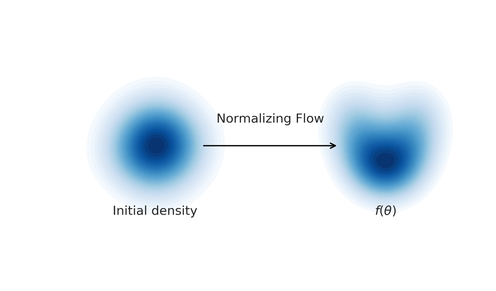
Furthermore, if one does not expect the posterior to look Gaussian (or a Gaussian mixture model), one can turn to “Normalizing Flows”.
A normalizing flow is a flexible transformation between probability distributions:

A normalizing flow learns an invertible dynamical model for samples of the distribution. Sample a Gaussian, and go forward through the dynamical model to sample the learned distribution. Invert the model and go backward from a sample to the compute the likelihood.
Each step is autoregressive^ (=change in y depends on x, followed by change in x depends on y), allowing it to be invertible. The invertibility implies normalization, since we aren’t creating additional Monte Carlo samples.
If you learn the dynamics with a flexible model, like a neural network, you can actually model an arbitrary distribution. This is great for non-Gaussian distributions.
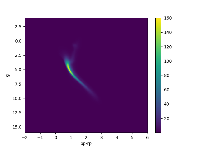
For an astronomy example, check out this paper where we learn an accurate data-driven HR diagram directly from Gaia data with a normalizing flow. No theory and no assumption of Gaussianity.
Modern LFI techniques model \(P(\theta|x)\) as normalizing flows, to learn very flexible likelihoods. Here is the procedure:
- Optionally learn a compression of \(x\) to a smaller number of features.
- Learn a normalizing flow that maximizes \(P(\theta|x)\) over examples. We can then both sample from and evaluate the posterior of \(\theta\) given samples.
PyTorch quick start
Here, I introduce PyTorch, which is used as the backend for sbi. It’s more of
an introduction for scientists who don’t do machine learning typically, as I
want to encourage them to use these DL frameworks for scientific computing.
I think it’s wise to write your array-based simulations by piggy-backing
on a package which is relied on and optimized by a
many-billion dollar industry.
Feel free to skip this section if you are comfortable with PyTorch.
In [2]:
import torch
import numpy as np
PyTorch is like numpy in syntax, but adds: vectorization, GPU-acceleration, and autodifferentiation. It also has deep learning kits. Let’s do some linear algebra:
Instead of np.array, we use torch.tensor:
In [3]:
np.array([5., 3.]), torch.tensor([5., 3.])(array([5., 3.]), tensor([5., 3.]))
But we can pass data back and forth between numpy and torch like so:
In [4]:
x = np.array([10., 5., 1.])
y = torch.tensor(x)
z = np.array(y)
x, y, z
(array([10., 5., 1.]),
tensor([10., 5., 1.], dtype=torch.float64),
array([10., 5., 1.]))
Create a vector of 10 zeros:
In [5]:
x = torch.zeros(10)
x
tensor([0., 0., 0., 0., 0., 0., 0., 0., 0., 0.])
Add 1 to each element:
In [6]:
x + 1tensor([1., 1., 1., 1., 1., 1., 1., 1., 1., 1.])
Generate random numbers:
In [7]:
x = torch.randn(10)
x
tensor([ 0.8344, 0.1738, -0.7568, 0.1369, 0.1513, 0.0052, 0.2035, -1.2633,
-0.9020, 0.8539])
Do some basic operations, all with numpy syntax:
In [8]:
torch.cos(x), torch.log(torch.abs(x) + 1), torch.sum(x), x.std()(tensor([0.6716, 0.9849, 0.7271, 0.9906, 0.9886, 1.0000, 0.9794, 0.3027, 0.6201,
0.6571]),
tensor([0.6067, 0.1602, 0.5635, 0.1283, 0.1409, 0.0052, 0.1852, 0.8168, 0.6429,
0.6173]),
tensor(-0.5630),
tensor(0.7062))
Now, let’s do stuff on the GPU:
In [9]:
x = torch.randn((100, 100))

# Move to GPU:
x = x.cuda()
x
tensor([[-1.3129, -0.6998, -0.1639, ..., -0.2922, 0.9799, 0.2962],
[ 0.3176, -1.4630, 0.5830, ..., 0.2930, 0.2625, 0.1684],
[-2.1551, 2.2514, -0.8173, ..., -2.6452, 0.9850, -0.2836],
...,
[ 1.1963, 0.5753, 1.4584, ..., -0.1940, -0.6713, 0.2051],
[ 0.6018, -0.7904, -0.4918, ..., 0.4556, 0.2463, -1.3733],
[ 0.9120, 0.4902, -0.9096, ..., 0.2018, 0.1721, -0.2624]],
device='cuda:0')
So the vector is on the GPU. We can do vector operations all on the GPU now:
In [10]:
y = x**3 + torch.cos(x) - x.mean()
y
tensor([[ -2.0060, 0.4243, 0.9842, ..., 0.9347, 1.5000, 0.9844],
[ 0.9840, -3.0218, 1.0350, ..., 0.9845, 0.9858, 0.9926],
[-10.5596, 10.7842, 0.1401, ..., -19.3868, 1.5106, 0.9393],
...,
[ 2.0799, 1.0315, 3.2161, ..., 0.9759, 0.4825, 0.9897],
[ 1.0443, 0.2117, 0.7645, ..., 0.9946, 0.9868, -2.3916],
[ 1.3727, 1.0020, -0.1365, ..., 0.9899, 0.9923, 0.9497]],
device='cuda:0')
And move back to the CPU like so:
In [11]:
z = y.cpu()
z
tensor([[ -2.0060, 0.4243, 0.9842, ..., 0.9347, 1.5000, 0.9844],
[ 0.9840, -3.0218, 1.0350, ..., 0.9845, 0.9858, 0.9926],
[-10.5596, 10.7842, 0.1401, ..., -19.3868, 1.5106, 0.9393],
...,
[ 2.0799, 1.0315, 3.2161, ..., 0.9759, 0.4825, 0.9897],
[ 1.0443, 0.2117, 0.7645, ..., 0.9946, 0.9868, -2.3916],
[ 1.3727, 1.0020, -0.1365, ..., 0.9899, 0.9923, 0.9497]])
PyTorch also lets you do autodifferentiation, which is a big part of deep learning. Let’s look at the gradient of \(\sum_i \cos(x_i)^2\):
In [12]:
def my_func(x):
    return (torch.cos(x)**2).sum()
First, we make our variable know that it should record gradients as it is
operated upon with the requires_grad flag:
In [13]:
x = torch.tensor([np.pi/4, np.pi/8])
x.requires_grad = True
Now, we take the analytic gradient at each of \(x=({\pi \over 4}, {\pi \over 8})\), which is \(-2 \cos(x) \sin(x)\):
In [14]:
torch.autograd.grad(my_func(x), x)(tensor([-1.0000, -0.7071]),)
We can also do this all on the GPU! We can also do higher-order derivatives by repeatedly calling grad.
In [15]:
y = x.cuda()
torch.autograd.grad(my_func(y), y)
(tensor([-1.0000, -0.7071], device='cuda:0'),)
With gradient information, one can do gradient descent operation on a model
using torch.optim.SGD:
In [16]:
torch.optim.SGD;One can write a class that inherits from torch.nn.Module, declares
torch.nn.Parameters(...) around its parameters, and then torch.optim.SGD can
optimize those. This is how all deep learning works: gradient-based optimization
of some highly-flexible differentiable model.
PyTorch is used as the backend for SBI. Let’s now move to likelihood-free inference.
Likelihood-free Inference:
Say that there is the following true model—a 2D Gaussian with known width:
The true vector for the Gaussian is \(\mu = (3, -1.5)\), which we are unaware of. We make 5 observations and attempt to reconstruct a posterior over \(\mu\).
The likelihood of this model is given by
which gives us a way to recover the parameter given data and a prior: \(P(\mu|x) \sim P(x|\mu) P(\mu)\).
But now, say that we don’t know this likelihood. Pretend we are not given the likelihood of a Gaussian. We only know how to draw samples from a Gaussian: this is our “simulation.”
How can we compute a distribution over \(\mu\), without a likelihood?
For LFI, you need to provide two ingredients:
- a prior distribution that allows to sample parameter sets (your guess at \(\mu\))
- a simulator that takes parameter sets and produces simulation outputs (samples of a Gaussian with a given \(\mu\))
For example, let’s pretend we have a reasonable idea that each \(\mu_i\) is within \([-5, 5]\) with uniform probability. We also have our simulator that generates samples of a Gaussian.
sbi tutorial:
sbi provides a simple interface to run simulation-based inference.
In [17]:
import torch
import sbi.utils as utils
from sbi.inference.base import infer
Let’s write out our uniform prior:
In [18]:
prior = utils.BoxUniform(
    low=torch.tensor([-5., -5.]),
    high=torch.tensor([5., 5.])
)
This will be used to generate proposals for \(\mu\).
Now, let’s write out our simulator for a given \(\mu\):
In [19]:
def simulator(mu):
    # Generate samples from N(mu, sigma=0.5)

    return mu + 0.5 * torch.randn_like(mu)
This simulator will take an estimate for \((\mu_1, \mu_2)\), and output a “simulation result” as a random sample of a Gaussian. If we pick the right \(\mu_1, \mu_2\), the output of the simulator will be close to our observed data.
Step 1: Let’s learn a likelihood from the simulator:
We use sbi to record 200 simulations from the above function, and fit
the joint surface of \(\mu_1, \mu_2, x_1, x_2\) with a neural network using
one of the three LFI algorithms.
This will be a bit slow because we are training the neural network on a CPU:
In [20]:
num_sim = 200
method = 'SNRE' #SNPE or SNLE or SNRE
posterior = infer(
    simulator,
    prior,
    # See glossary for explanation of methods.
    #    SNRE newer than SNLE newer than SNPE.
    method=method,
    num_workers=-1,
    num_simulations=num_sim)
Neural network successfully converged after 57 epochs.
Now we have a neural network that acts as our likelihood!
Step 2, let’s record our 5 “observations” of the true distribution:
In [21]:
n_observations = 5
observation = torch.tensor([3., -1.5])[None] + 0.5*torch.randn(n_observations, 2)
In [22]:
import seaborn as sns
from matplotlib import pyplot as plt
/usr/local/lib/python3.6/dist-packages/statsmodels/tools/_testing.py:19: FutureWarning: pandas.util.testing is deprecated. Use the functions in the public API at pandas.testing instead.
import pandas.util.testing as tm
Here’s the data:
In [23]:
sns.scatterplot(x=observation[:, 0], y=observation[:, 1])
plt.xlabel(r'$$x_1$$')
plt.ylabel(r'$$x_2$$')
plt.xlim(-10, 10)
plt.ylim(-10, 10)
plt.show()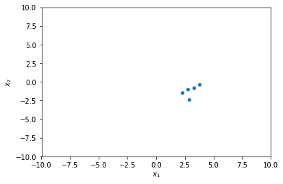
We can now use our learned likelihood (a neural network) to do inference on \(\mu\)!
Step 3, Inference
Sampling
We can sample the posterior for a single datapoint like so:
In [24]:
samples = posterior.sample((200,), x=observation[0])Tuning bracket width...: 100%|██████████| 50/50 [00:00<00:00, 58.36it/s]
Generating samples: 100%|██████████| 20/20 [00:00<00:00, 20.97it/s]
Generating samples: 100%|██████████| 200/200 [00:09<00:00, 20.73it/s]
And then plot this (it should look approximately Gaussian):
In [25]:
log_probability = posterior.log_prob(samples, x=observation[0])
out = utils.pairplot(samples, limits=[[-5,5],[-5,5]], fig_size=(6,6), upper='kde', diag='kde')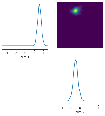
For multiple observations, one should compute the total log-probability (see below), and MCMC.
Computing log-probability:
Let’s create a grid of \(\mu\) close to the expected value of \((3, -1.5)\), and calculate the total log likelihood for each value:
In [26]:
import numpy as np

bounds = [3-1, 3+1, -1.5-1, -1.5+1]

mu_1, mu_2 = torch.tensor(np.mgrid[bounds[0]:bounds[1]:2/50., bounds[2]:bounds[3]:2/50.]).float()

grids = torch.cat(
    (mu_1.reshape(-1, 1), mu_2.reshape(-1, 1)),
    dim=1
)
In [27]:
grids.shapetorch.Size([2500, 2])
Let’s calculate the log probability across the grid. One can usually use
posterior.log_prob, but one can also vectorize it as follows:
In [28]:
if method == 'SNPE':
    log_prob = sum([
        posterior.log_prob(grids, observation[i])
        for i in range(len(observation))
    ])
else:
    log_prob = sum([
        posterior.net(torch.cat((grids, observation[i].repeat((grids.shape[0])).reshape(-1, 2)), dim=1))[:, 0] + posterior._prior.log_prob(grids)
        for i in range(len(observation))
    ]).detach()

prob = torch.exp(log_prob - log_prob.max())
plt.figure(dpi=200)
plt.plot([2, 4], [-1.5, -1.5], color='k')
plt.plot([3, 3], [-0.5, -2.5], color='k')
plt.contourf(prob.reshape(*mu_1.shape), extent=bounds, origin='lower')
plt.axis('scaled')
plt.xlim(2+0.3, 4-0.3)
plt.ylim(-2.5+0.3, -0.5-0.3)
plt.title('Posterior with learned likelihood\nfrom %d examples of'%(num_sim)+r' $$\mu_i\in[-5, 5]$$')
plt.xlabel(r'$$\mu_1$$')
plt.ylabel(r'$$\mu_2$$')
Text(0, 0.5, '$$\\mu_2$$')
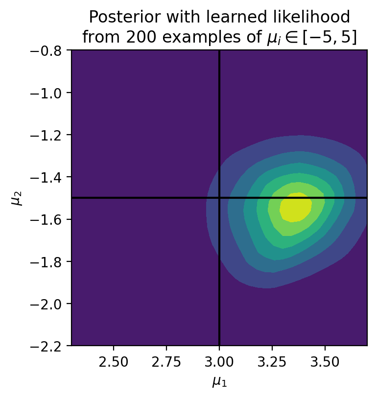
Now, this was a simple example and we could have written out an explicit likelihood. But the real power of Likelihood-Free Inference comes for high dimensional and complicated distributions, when there is no explicit analytic likelihood available. The exact same algorithm as above can simply be scaled up to a higher dimensional space.
Let’s compare to the true likelihood:
In [29]:
true_like = lambda x: -((x[0] - mu_1)**2 + (x[1] - mu_2)**2)/(2*0.5**2)
log_prob = sum([true_like(observation[i]) for i in range(len(observation))])
plt.figure(dpi=200)
prob = torch.exp(log_prob - log_prob.max())
plt.plot([2, 4], [-1.5, -1.5], color='k')
plt.plot([3, 3], [-0.5, -2.5], color='k')
plt.contourf(prob.reshape(*mu_1.shape), extent=bounds, origin='lower')
plt.axis('scaled')
plt.xlim(2+0.3, 4-0.3)
plt.ylim(-2.5+0.3, -0.5-0.3)
plt.title('Posterior with\nanalytic likelihood')
plt.xlabel(r'$$\mu_1$$')
plt.ylabel(r'$$\mu_2$$')
Text(0, 0.5, '$$\\mu_2$$')
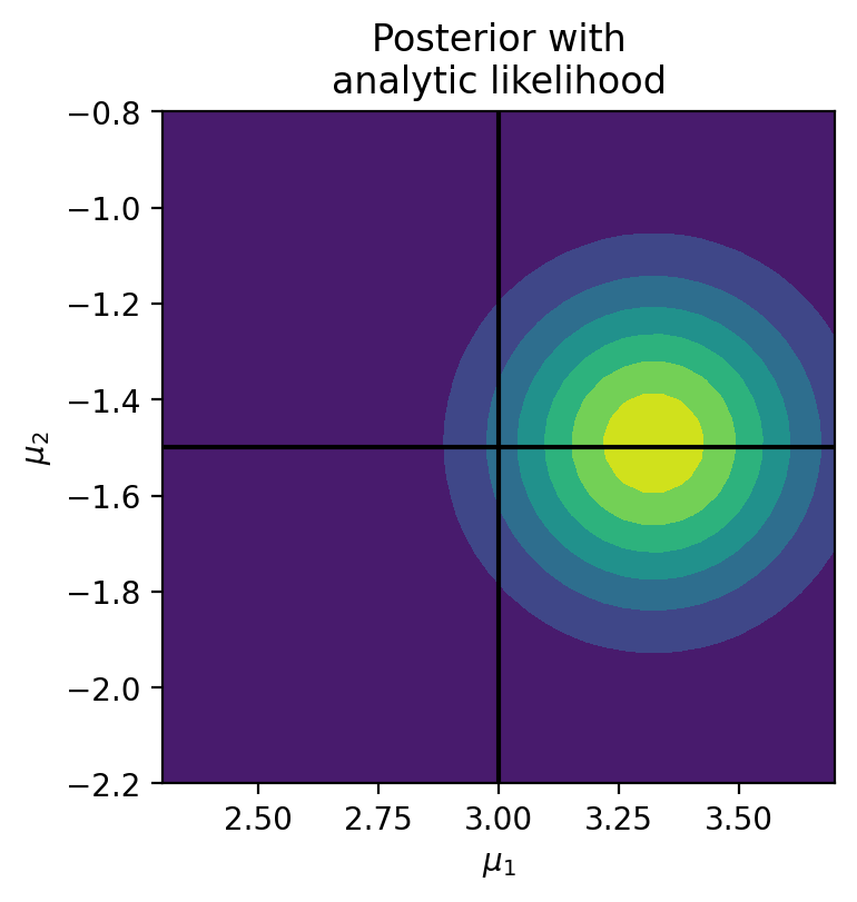
Not bad considering we only used \(200\) examples to learn the likelihood, which is a complex function \(\propto (x_1 - \mu_1)^2 + (x_2 - \mu_2)^2\)! The more simulations you use (much faster to train with GPUs), the more accurate the likelihood will be.
Emphasis:
LFI is a very general approach that will eventually be used everywhere in astrophysics where we don’t have clear likelihoods. To help give examples of what it could do:
- Photo-z: parameter is z, you then generate some SEDs - that is your
“simulator”. Then use
sbito compare to data. You get a posterior over z. - Galaxy images: parameters are galaxy properties, orientation, distance, you
then simulate some images of galaxies. You then use
sbito infer the galaxy properties.- Here, one would probably want to use an autoencoder to first compress the images to vectors describing the properties.
- The likelihood is then learned over that vector.
Answers to questions during my tutorial:
- Your simulator does not need to be differentiable. All you need is the input and output.
- LFI was invented for very expensive & high-dimensional simulations; the toy example we did was a 2D Gaussian just to help with building intuition.
- The range of parameters which you simulate is linked to the accuracy of the likelihood you learn (the closer the parameters you simulate from are to the true parameters, the less the model needs to interpolate). We chose a wide prior of \(\mu_i \in [-5, 5]\), but a tighter prior would result in a more accurate likelihood. (i.e., generally you want your simulations to have realistic parameters).
- This may sound strange for those who have not done deep learning, but the time difference between our 2-D case and a 100-D case is small, as the internal model (“hidden layers”) is the same for both.
Methods available:
SNPE = sequential neural posterior estimation = https://papers.nips.cc/paper/6728-flexible-statistical-inference-for- mechanistic-models-of-neural-dynamics.pdf.
Outputs as a Gaussian mixture model. Difference: generates parameter samples from a learned proposal that make generated data closer to the observed data.
SNLE = sequential neural likelihood estimation = http://proceedings.mlr.press/v89/papamakarios19a/papamakarios19a.pdf.
Train a likelihood as a conditional normalizing flow. Will learn summary statistics internally.
SNRE = Sequential Neural Ratio Estimation = https://arxiv.org/abs/1903.04057.
Targets the likelihood ratio between two choices of parameters.