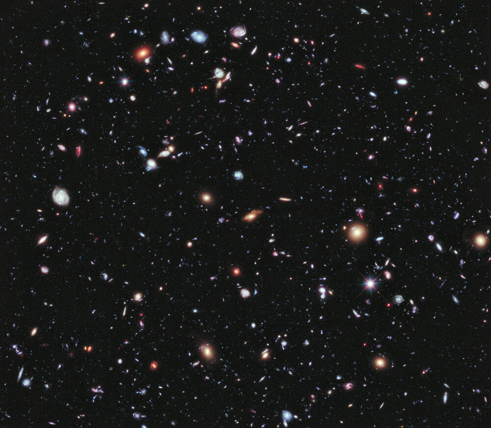
 The Hubble eXtreme Deep Field, showing over 5,500 galaxies
Unsupervised Resource Allocation with Graph Neural Networks
Paper authors: Miles Cranmer, Peter Melchior, Brian Nord
At its core, science is a remarkably simple process. Design a model to describe how something works. Test the predictions. Repeat.
Through this loop—whether applied explicitly or implicitly—we continuously deepen our understanding of the universe’s workings, from the physical intuition we learned as children playing with toys to the dynamical equations we’ve discovered to describe the evolution of the universe. All of this understanding has resulted from an application of the scientific process.
Now, what if we could automate this process? What if we could automate scientific discovery?
The research loop of astronomy is no different: one designs a physical model for some phenomenon, collects data to test the model, then analyzes it against a competing prediction. However, selecting sources to observe and then engineering an analysis pipeline is very nontrivial. This is especially true when the phenomenon is multiscale and involves interacting sources, such as galaxies.
In this paper, we present an algorithm to automate and improve the source selection and analysis steps in an unsupervised way. This observational schedule is learned from scratch. No labels are needed to tell the network which phenomena are useful tracers, nor how the observed properties relate to the parameter of interest.
This is actually a problem encountered in many disciplines across both academia and industry under different names: given several options, how does one distribute a finite amount of resources among them to optimize a global utility? We often have an unknown relationship between these targets and the utility. We call this: “Unsupervised Resource Allocation.”
For any real-world problem of this nature, these options are not independent. Their properties are correlated with each other, and the interactions between them may influence the global utility. Thus, we use Graph Neural Networks as our base architecture, due to their many useful properties: they can model interactions explicitly via edges, they naturally have permutation equivariance, and they can also be easily modified to include common physical symmetries such as translational equivariance. They are also uniquely interpretable: for some physical problems, they can be completely and explicitly converted to a symbolic expression.
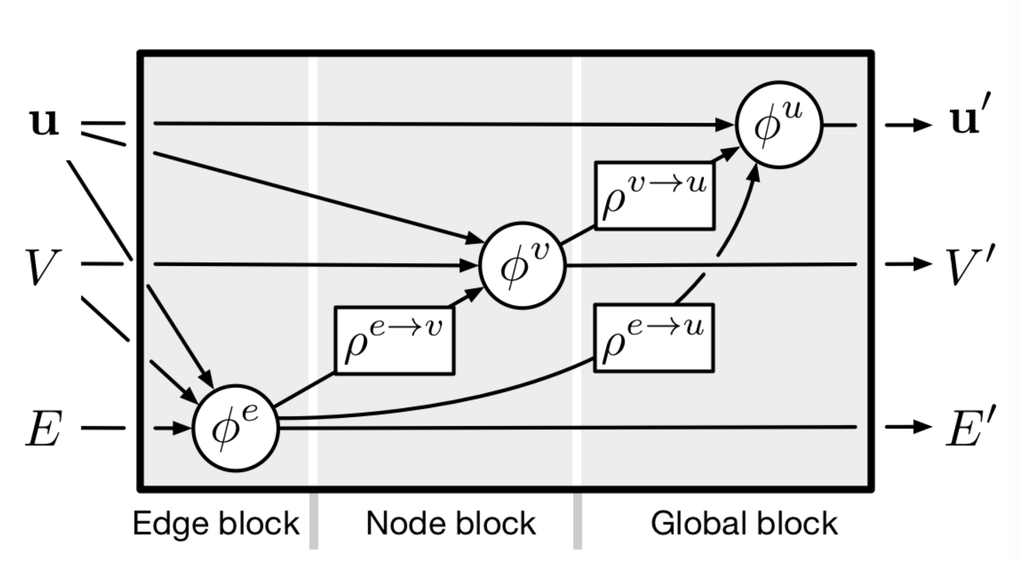
A Graph Neural Network (GNN) operates on a graph—a tuple \(G=(u, V, E)\), for \(u\) a global property, \(V\) a set of nodes, and \(E\) a set of edges and edge-specific attributes. In the notation of Peter Battaglia’s GNN review, a single GNN “block” can be represented as
 |
|---|
| A single graph neural network “block”, which outputs updated global, nodes, and edges. (source) |
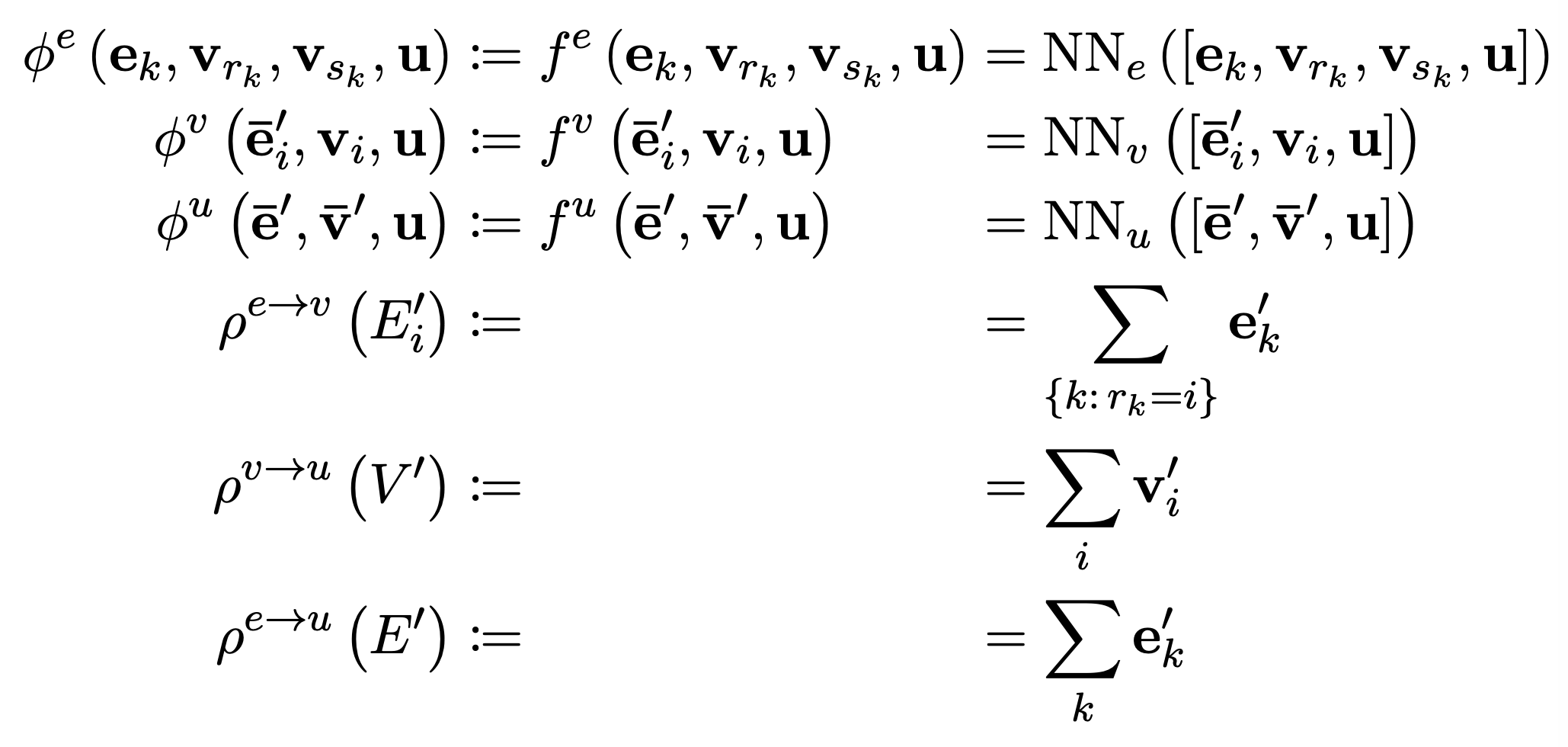
Each \(\phi\) is commonly a multi-layer perceptron, or in the case of Graph Convolutional Networks, closer to a single matrix multiplication. Each \(\rho\) is a permutation-invariant pooling operator, such as an element wise sum. For multiple message-passing steps, one stacks additional GNNs to the right. One commonly encodes features into a high-dimensional latent space before passing through a GNN block.
 |
|---|
| The equations describing a common implementation of a graph neural network block.(source) |
One can derive variants of GNNs by removing elements from this schematic - e.g., a DeepSet is found by removing all parts with the edge set \(E\) from this diagram.
We use two GNNs in our method: one GNN, which acts to predict the resources allocated to a particular target, and the second GNN, which acts as a stand-in model for a differentiable analysis pipeline. We train these together - the second GNN will learn to become a near-optimal noise-robust prediction network, and via their joint optimization, the first GNN will learn to produce a near-optimal allocation strategy.
 |
|---|
| Our proposed algorithm for unsupervised resource allocation. |
We work with three message-passing steps in our GNNs, with sum-pools for the allocation GNN [motivation: the network needs to be aware of the total allocation], and mean-pools for our inference GNN [motivation: Cosmological properties are an intrinsic (averaged) property, not an extrinsic (summed) property]
In astronomy, the resource in question is the observing time at a world-class telescope. For an individual observing program, astronomers will write “observing proposals” for telescope time which convince reviewers that their particular allocation is worthwhile. Here we propose a machine learning technique to automate this process. With a simulated model for the observed phenomenon, and differentiable model of the telescope, we show how our algorithm can learn an optimal allocation strategy: for large surveys, our learned allocation strategy outperforms traditional heuristics-based methods, even when those methods are given the same learned analysis GNN.
 |
|---|
| Our resource allocation model implemented for an astronomy application, compared with a standard astronomical pipeline. |
We train our model to produce an optimal selection of dark matter halos in the Quijote simulations that produce the most accurate prediction of \(\Omega_m\). We generate random fields of galaxies which look like the following:
 |
|---|
| An example field of galaxies from which our resource allocation much allocate observing time to. Size of each dot correlates with mass, and color shows redshift. |
The right figure shows how we connect nearby galaxies with edges to input to our graph network. Each halo has two features—mass and redshift—which we initially add significant noise to. The allocated resources are parametrized as observing time of a telescope, and we convert this observing time to a reduced amount of noise in the mass and redshift for each halo via a simulated spectroscopic pipeline. Thus, the resource allocation GNN acts to remove a limited amount of noise from observations. Following this, the “inference GNN” uses the data, now with reduced noise, and computes a prediction—in this case, \(\Omega_m\).
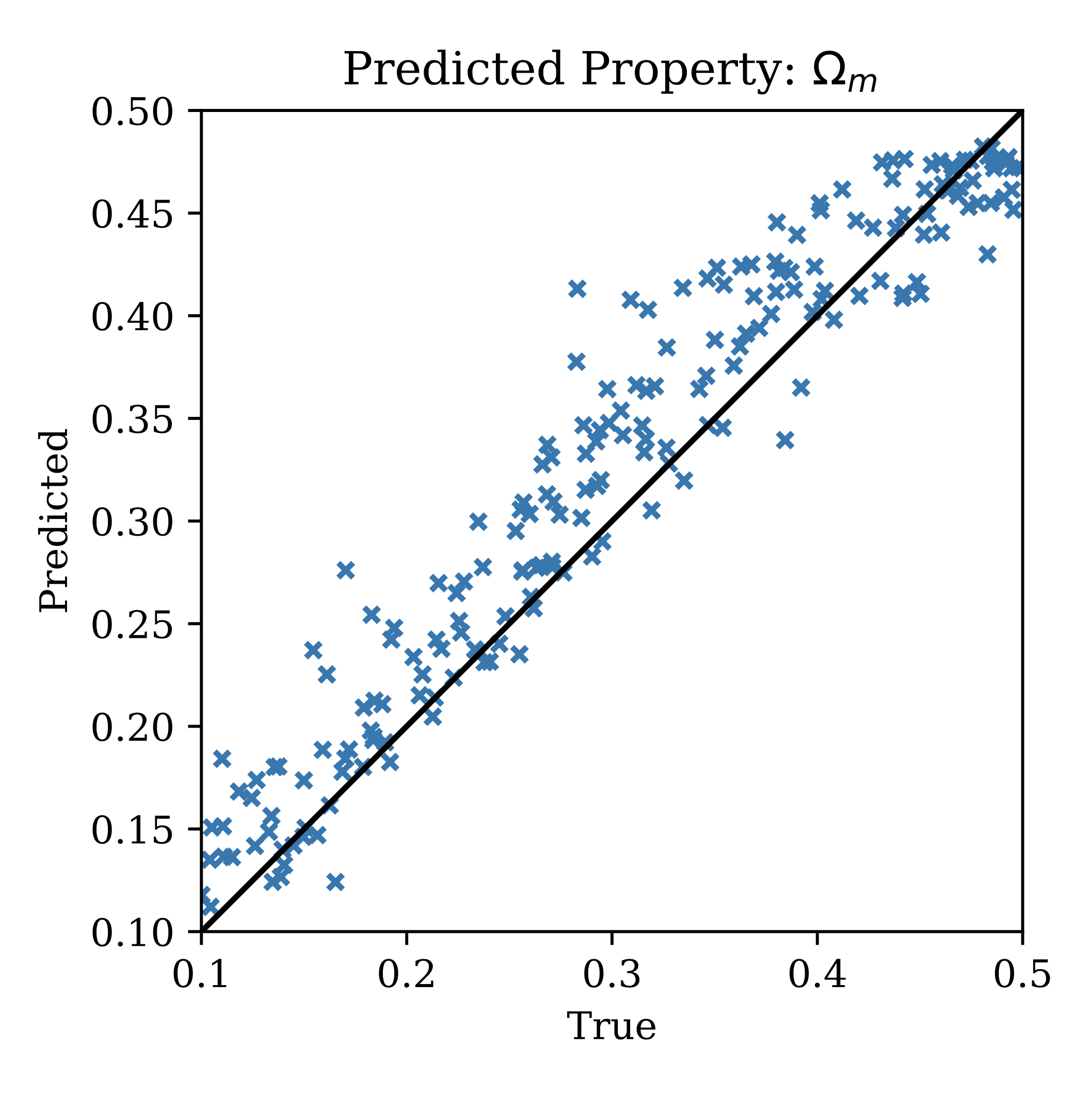
We can plot out the predictions versus the true \(\Omega_m\) values on a test set, and then compare the predictions to two common strategies for resource allocation in astronomy:
 |
|---|
| Predicted vs true \(\Omega_m\) from our allocation-analysis pipeline, on our small simulated datasets. |
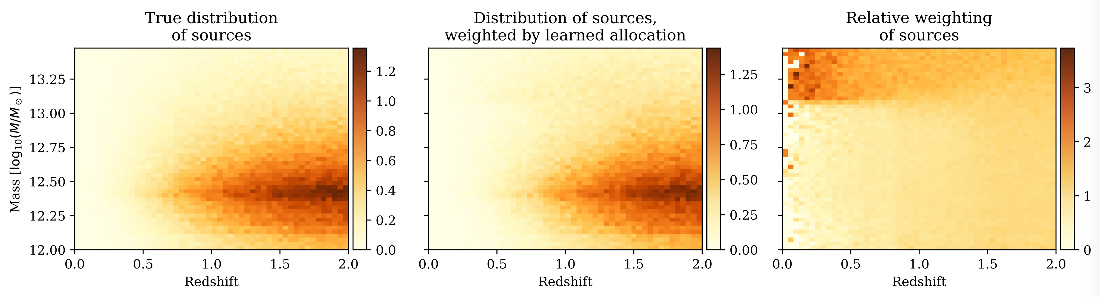
Despite the luminosity threshold and beta distribution strategies being tuned with a genetic algorithm, and using the same inference GNN, they tend to perform worse than the allocation GNN. We can also study how our model has learned to allocate resources, by looking at a histogram of sources, weighted by resource allocation:
 |
|---|
| The resource allocation GNN’s learned relative importance of galaxies as a function of mass-redshift. |
As can be seen in the right plot, our model has learned that high-mass, low-redshift galaxies offer the best value per allocated time, so it selects them frequently relative to other areas of parameter space.
We look forward to applying our technique to more problems in the future, as well as implementing it for various astronomical pipelines.
Please let us know on Twitter or via email if you have any questions!