A Bayesian neural network predicts the dissolution of compact planetary systems

Paper Inference Code Training Code Interactive Notebook

Paper authors: Miles Cranmer, Daniel Tamayo, Hanno Rein, Peter Battaglia, Samuel Hadden, Philip J. Armitage, Shirley Ho, David N. Spergel

The heavenly motions are nothing but a continuous song for several voices, to be perceived by the intellect, not by the ear; a music which ... sets landmarks in the immeasurable flow of time — Johannes Keppler

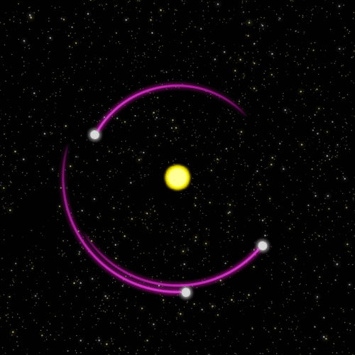
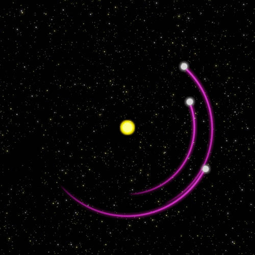
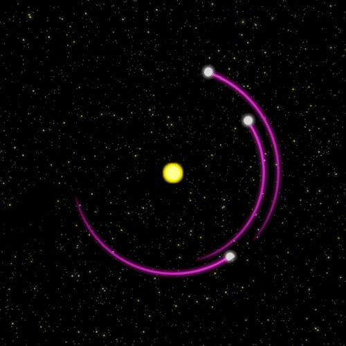
Three planets dance around a star in the vacuum of space. At each moment, they exert a gravitational pull on one another, obeying a simple rule to meticulous precision.

Though elementary, this system produces very complex patterns. Over long timescales it becomes impossible to predict in detail. This represents a variant of the three-body problem, the prototypical example of a chaotic system. For a broad range of planetary systems, shifting one planet by a centimeter could maintain the system’s stability for the remainder of its star’s lifetime, or result in an early ejection of its neighbor.

Such phenomena—where incredible complexity emerges from simple systems—remains what I consider the most beautiful aspect of all physics. This complexity arranges our universe as a sort of mysterious architect—in our case, setting up a chain of collisions, assembling the Earth from smaller bodies.

Can we predict what these chaotic systems will do far in the future? For an exoplanet system, what necessary ingredients in an orbital configuration produce stability? What systems go unstable and experience a collision or ejection, and at what time will this occur? Being able to answer these questions will help improve our understanding of planet formation, and help constrain the parameters of observed exoplanet systems.

Though visually similar, these systems will go unstable at times which are orders of magnitude different.

Luckily, there exist limits to the chaotic nature of compact planetary systems (Hussain & Tamayo, 2020). For each system, a particular range of times determines when it could go unstable, and it should theoretically be possible to constrain this range. Consider this: though we cannot predict a single toss of a fair coin, we can still predict the accumulation of tosses. Though we cannot predict every single gravitational interaction between planets, we should be able to predict the accumulation of many planetary interactions required to reach collision trajectories.

Problem

However, despite over three centuries of effort, no closed-form solutions exist for predicting the times over which a general planetary configuration may become unstable. One can simulate these dynamical systems, but the price of 10 CPU hours per initialization means that numerically exploring stable parameter regimes using \(\sim 10^6\) different systems remains computationally intractable.

In recent years, significant theoretical work (e.g., Sessin & Ferraz-Mello, 1984; Cincotta et al., 2003; Deck et al., 2013; Hadden, 2019) has motivated metrics for instability in planetary systems. These metrics find use in simple machine learning models to compute the probability a system will remain stable a set time, using a simulated training dataset: Tamayo et al. (2020).

In our new paper, we learn instability metrics from scratch, using only the raw orbital parameters of a planetary system. Our model can accurately predict not only if, but also when a compact planetary system with three or more planets will go unstable. Despite lacking embedded domain knowledge, our model’s learned metrics improve predictive accuracy. It also shows robust generalization to a 5-planet dataset, even though we trained it only on 3-planet systems in a different part of parameter space.

Inductive Biases and Bayesian Deep Learning

How did we get this to work? Early on, we encountered significant difficulty tackling this problem with models in the standard machine learning toolkit such as LSTMs, Gaussian Processes, and CNNs. Part of the issue is due to the existence of “resonances” in planetary systems: these points in parameter space allow tiny shifts in an input parameter to change the result by orders of magnitude. Such sharp boundaries do not typically exist in common machine learning datasets.

In deep learning, the “inductive bias” of a model often determines its success. The inductive bias can be loosely defined as the algorithmic motif of a neural network architecture. A convolutional neural network convolves filters over the pixels of an image. This gives us translational equivariance, and rough algorithmic similarity to a hand-engineered computer vision model, which might explain why CNNs remain the champion of computer vision models. Likewise, a graph neural network learns messages to pass between nodes on a graph. This inductive bias explains why graph nets dominate N-body problems: they show similar algorithmic structure to the physical model!

...common patterns in neural networks correspond to very natural, simple functional programs. These patterns are building blocks which can be combined together into larger networks. Like the building blocks, these combinations are functional programs, with chunks of neural network throughout. The functional program provides high level structure, while the chunks are flexible pieces that learn to perform the actual task within the framework provided by the functional program. These combinations of building blocks can do really, really remarkable things.

—Chris Olah on “A New Kind of Programming”

Our model has two essential inductive biases motivated by the problem:

Architecture. The first is in our architecture. Our model has a similar functional structure to successful ML models which use theoretically-derived metrics (spock.FeatureClassifier), but with added flexibility: hand-engineered functions are replaced with neural networks.

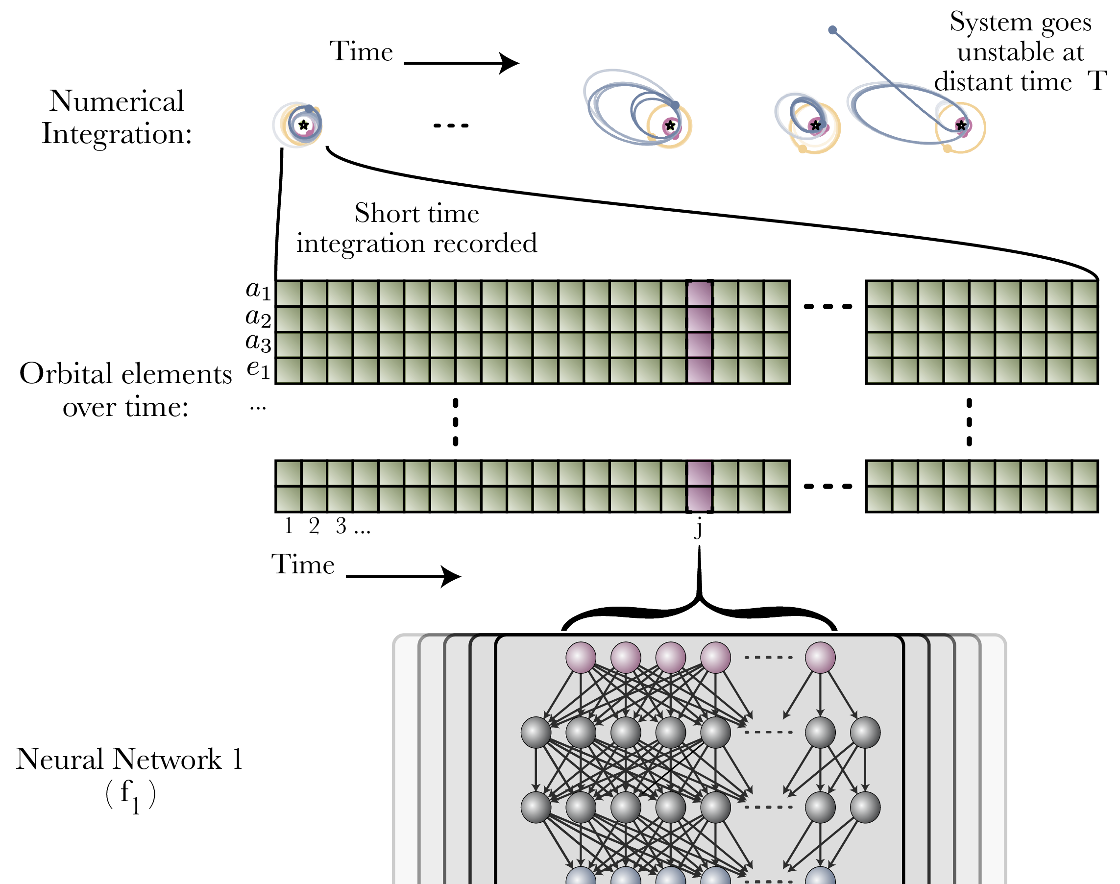
First, we record six orbital elements for each of three planets over 10,000 orbits, along with their mass.

A neural network takes these twenty-one parameters, and passes them through a learned mapping, converting them to another vector, for each time step. One can consider this essentially a learned coordinate transform.

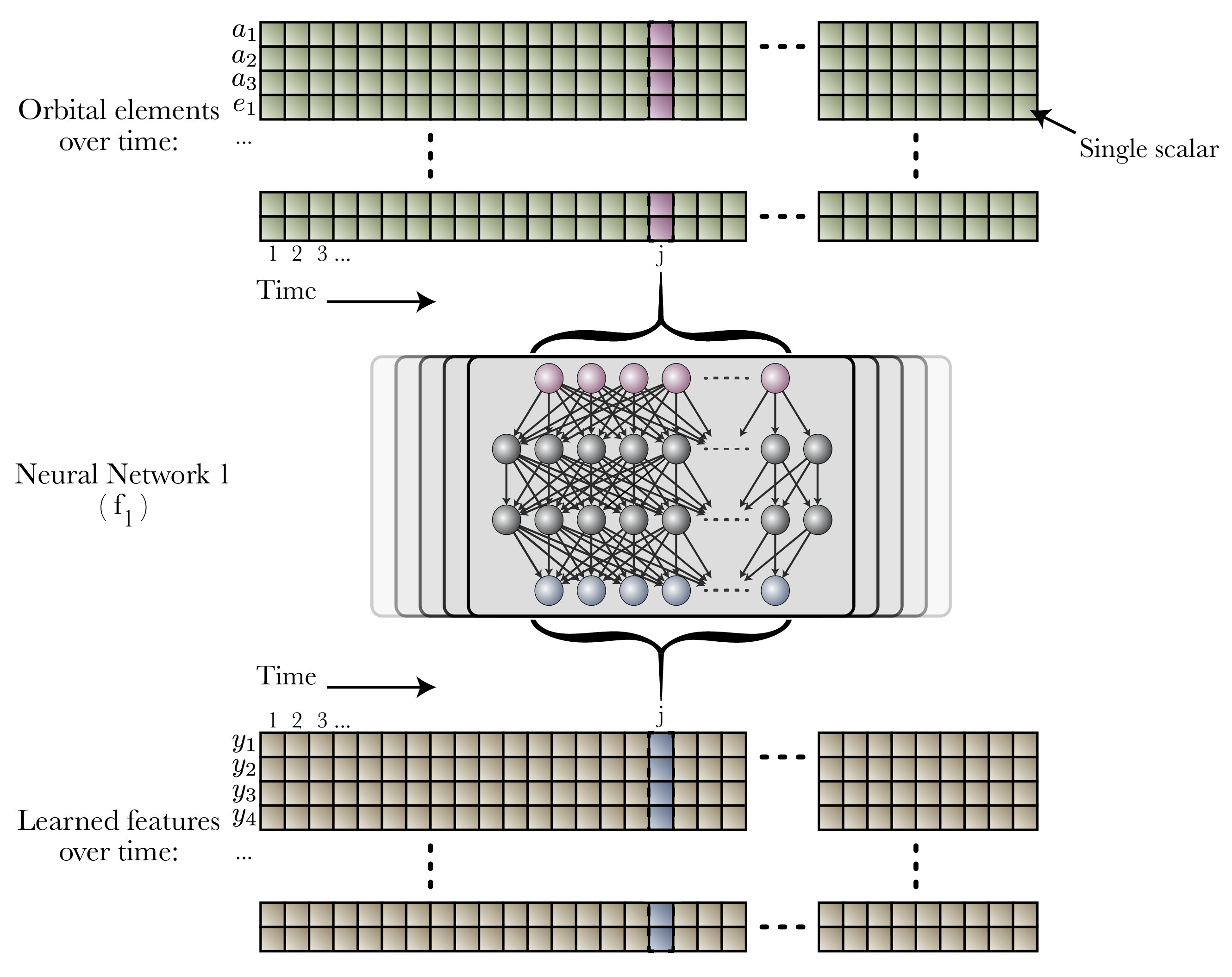
Next, we do a non-standard pooling operation of these features over the time axis: we compute both the mean and variance of these learned coordinates over time. Common metrics used in dynamics motivated this inductive bias: these metrics are often in the form of means and variances of instantaneous metrics over time.

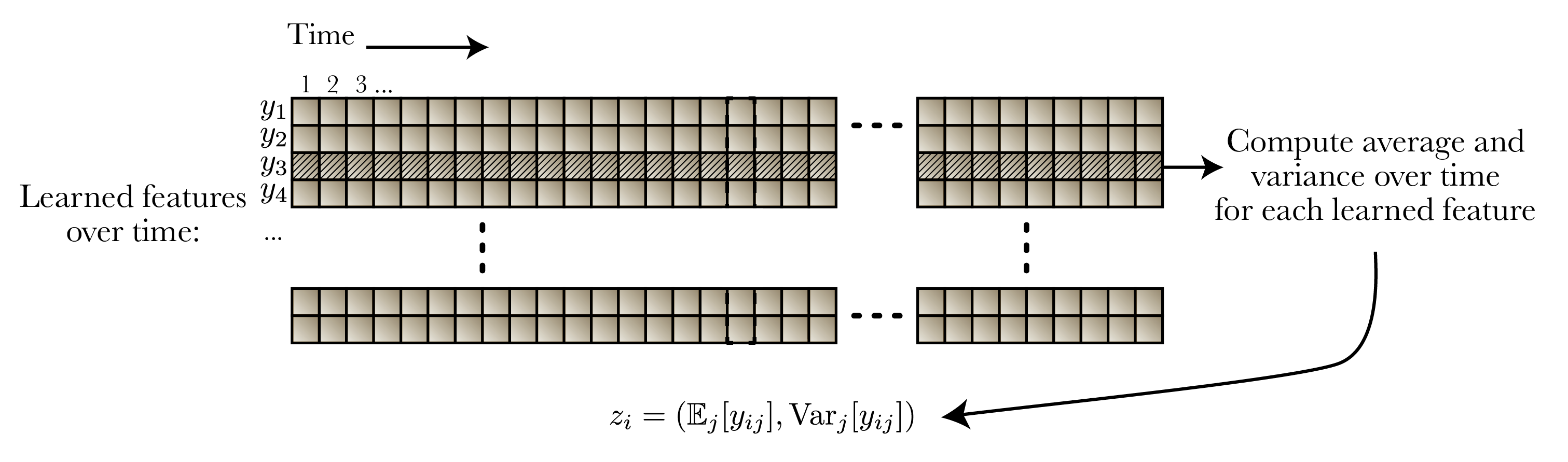
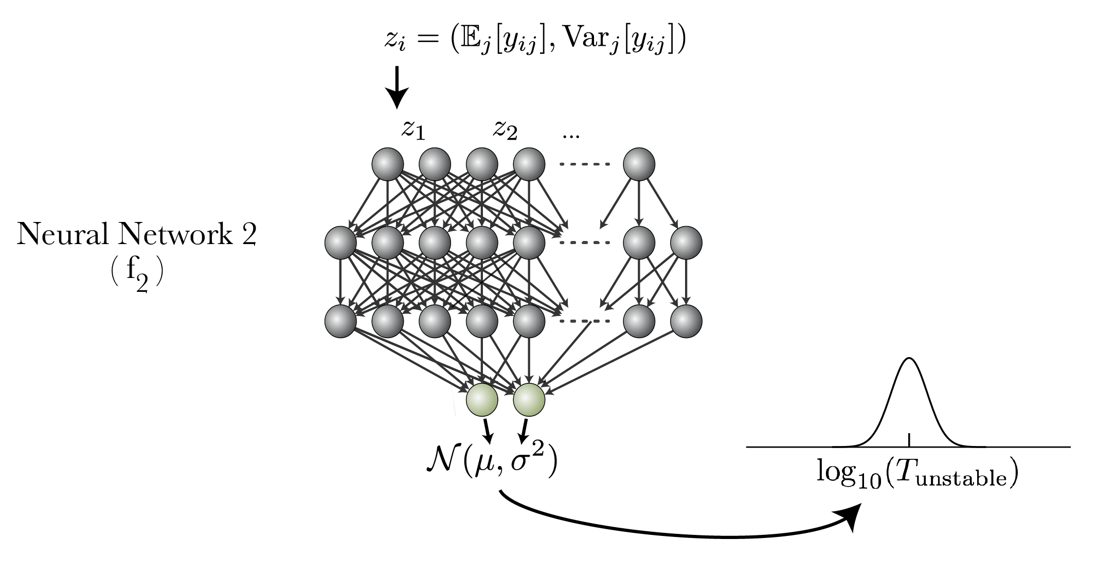
We then use these means and variances in a second neural network to predict instability time.

We train both neural networks at the same time with a single backpropagation. Accordingly, this means the metrics learned by the first network learns optimize the predictive power of the second network.

Parametrization.

The second inductive bias is in our parametrization. Because we deal with chaotic systems, we need to predict a distribution of instability times, not one point. We use Bayesian deep learning, and predict parameters of a lognormal distribution over instability time (the distribution motivated by Hussain & Tamayo, 2020), optimizing the log-likelihood of our simulation dataset.

Bayesian deep learning allows us to marginalize the parameters of our neural networks, giving us the ability to account for uncertainty due to extrapolation outside the training set:

Monte Carlo dropout—a variant of a Bayesian neural network Gal (2015).

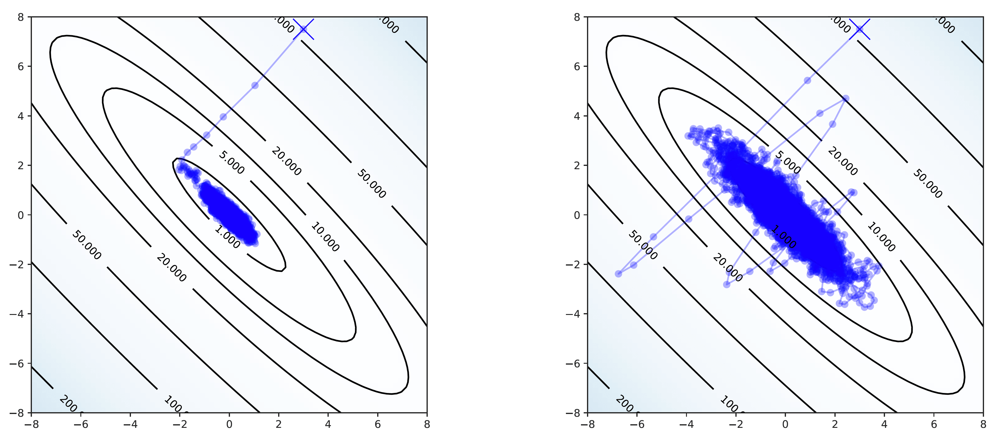
We use the Multimodal version of Stochastic Weight Averaging Gaussian (MultiSWAG; Wilson & Izmailov, 2020), a Bayesian neural network which beautifully exploits the connection between stochastic gradient descent and MCMC sampling (see Mingard et al., 2020 and Mandt et al., 2017). This framework models a distribution over the neural network’s weights with a low-rank Gaussian mixture model. This algorithm works as follows:

1. Train the model with stochastic gradient descent until the parameters settle into a local minimum of the weight posterior.
2. Increase the learning rate and continue training. This causes the optimizer to take a random walk in parameter space near the local minimum, which is assumed to look like a high-dimensional Gaussian.
3. Accumulate the average parameters along this random walk and a low-rank approximation of the covariance matrix.
4. The average parameters not only provide better generalization performance (stochastic weight averaging or SWA; Izmailov et al., 2018), but we have additionally fit a Gaussian to a mode of the parameter posterior. We can thus sample weights from this Gaussian to marginalize over parameters. This is SWAG (Maddox et al., 2019).
5. The next step is to repeat this process from a different random initialization of the parameters. This will find another mode of the parameter posterior.
6. Fit 30 different modes of the parameter space. We can then sample weights from multiple modes of the parameter posterior, which gives us a more rigorous uncertainty estimate. This is MultiSWAG (Wilson & Izmailov, 2020).

The trajectory of stochastic gradient descent near a minima, without momentum (left) and with momentum (right), from Maddox et al. (2019). Samples from this trajectory are used to fit a Gaussian to the mode of the parameter posterior.

Given this distribution of parameters, we can then make forward passes through our model to compute samples of an approximated posterior over instability time for a given system.

Results and Generalization

We train on systems with three planets orbiting a central star. Each is mapped to a short time series of 21 features recorded at 100 time steps, with a corresponding instability time. Our training dataset is dominated by resonant systems. We test our model on an unseen fraction of this resonant dataset, and a non-resonant dataset. Finally, we also test on systems with five planets in circular orbits, a vastly different section of parameter space compared to our training data.

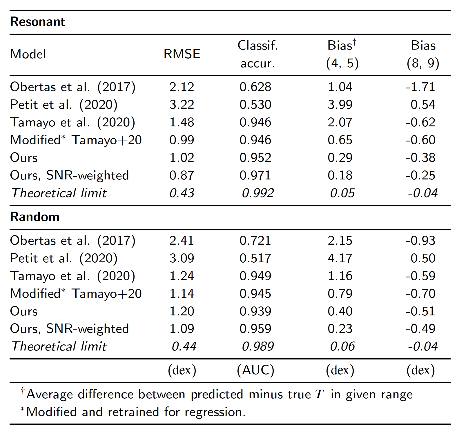
On the three planet train/test datasets, our model is two orders of magnitude more accurate than existing analytic estimators, while also reducing the bias of Tamayo et al. (2020) by a factor of three. Furthermore, all our estimates come with error bars, which allows one to detect sections of parameter space where the model’s predictions are uncertain.

A comparison of our model to other analytic and ML models on our test sets over resonant and non-resonant systems.

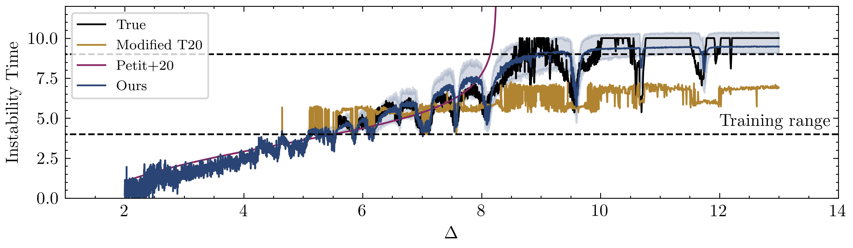
One can adapt our model to systems with more than three planets: (1) estimate the instability time for each trio of adjacent planets in the system, then (2) consider only the most unstable group (further details given in paper). Our model performs with this strategy on the 5-planet dataset, surpassing even models designed for that particular dataset. The remarkable thing about this is that these systems are completely unlike those trained on, yet this model still performs accurately.

Our model evaluated on a 5-planet dataset. Error bars show the 68% confidence interval, and the center line shows the median estimate. The x-axis shows increasing separation between planets.

API for Exoplanet Research

Our model is publicly available in the python package spock for efficiently computing instability estimates for planetary systems. Simulations which are parametrized with the rebound framework can be passed to the various functions to sample from our estimated posterior over instability time. An example is given below, which can be ran within our interactive online notebook here.

sims = []
masses = np.array([1, 2, 3, 4, 5]) * 1e-5
for m in masses:
    sim = rebound.Simulation()
    sim.add(m=1.)
    sim.add(m=m, P=1.)
    sim.add(m=m, P=1.3)
    sim.add(m=m, P=1.6)
    sims.append(sim)

median, lower, upper = deep_regressor.predict_instability_time(sims)

print(np.log10(median))

Which gives us:

[10.39, 9.60, 7.98, 7.13, 6.38]

meaning that our model’s median estimate is that systems with \(5\times 10^{-5}\) planetary mass relative to their star experience an instability at \(10^{6.38}\) orbits, \(4\times10^{-5}\) at \(10^{7.13}\) orbits, and so on.

Conclusion

We have described a probabilistic machine learning model—a Bayesian neural network—that can accurately predict a distribution over possible instability times for a compact multi-planet exoplanet system. Our model learns instability metrics from scratch, and demonstrates large improvements in predictive accuracy to existing analytic and ML-based methods.

Our model gives a computational speedup over N-body integrations of up to \(10^5\) times. This enables a broad range of applications: using stability constraints to rule out unphysical configurations and constrain orbital parameters, and for developing efficient terrestrial planet formation models.

Future work will also look at extracting analytic forms of this model from the perspective of existing dynamics theory, using methods from Cranmer et al., 2020.

Acknowledgements

Thanks to Dan Tamayo for helping me with this blog post, and Hanno Rein for creating the nice-looking gifs of some of our planetary systems used in training! Additional acknowledgements and references are given in the paper.

1. Book V, Ch. 7 as quoted in Arthur Koestler, The Sleepwalkers (1959)