Discovering Symbolic Models from Deep Learning with Inductive Biases

Paper Code Interactive Notebook

Paper authors: Miles Cranmer, Alvaro Sanchez-Gonzalez, Peter Battaglia, Rui Xu, Kyle Cranmer, David Spergel, Shirley Ho

At age 19, I read an interview of physicist Lee Smolin. One quote from the article would shape my entire career direction:

... let’s focus on quantum theory and relativity and their relation; if we succeed it will take generations to sort out the ramifications. We are still engaged in finishing the revolution Einstein started. This is, not surprisingly, a long process.

This statement disturbed me. The idea that a foreseeable limit exists on our understanding of physics by the end of my life was profoundly unsettling. I felt frustrated that I might never witness solutions to the great mysteries of science, no matter how hard I work.

But… perhaps one can find a way to tear down this limit. Artificial intelligence presents a new regime of scientific inquiry, where we can automate the research process itself. In automating science with computation, we might be able to strap science to Moore’s law and watch our knowledge grow exponentially rather than linearly with time.

When does a model become knowledge?

To automate science we need to automate knowledge discovery. However, when does a machine learning model become knowledge? Why are Maxwell’s equations considered a fact of science, but a deep learning model just an interpolation of data? For one, deep learning doesn’t generalize near as well as symbolic physics models. Yet there also seems to exist something that makes simple symbolic models uniquely powerful as descriptive models of the world. The origin of this connection hides from our view:

The miracle of the appropriateness of the language of mathematics for the formulation of the laws of physics is a wonderful gift which we neither understand nor deserve. We should be grateful for it and hope that it will remain valid in future research and that it will extend, for better or for worse, to our pleasure, even though perhaps also to our bafflement, to wide branches of learning.

—Eugene Wigner, The Unreasonable Effectiveness of Mathematics in the Natural Sciences

From a pure machine learning perspective, symbolic models also boast many advantages: they’re compact, present explicit interpretations, and generalize well. “Symbolic regression” is one such machine learning algorithm for symbolic models: it’s a supervised technique that assembles analytic functions to model a dataset. However, typically one uses genetic algorithms—essentially a brute force procedure as in Schmidt & Lipson (2009) or our open-source implementation PySR—which scale poorly with the number of input features. Therefore, many machine learning problems, especially in high dimensions, remain intractable for traditional symbolic regression.

Symbolic regression using a genetic algorithm. A binary tree of operators and variables represents an equation. Mutations and crossovers iterate on and combine the best models. Source.

On the other hand, deep learning proves extraordinarily efficient at learning in high-dimensional spaces, but suffers from poor generalization and interpretability. So, does there exist a way to combine the strengths of both?

Method

We propose a technique in our paper to do exactly this. In our strategy, the deep model’s job is not only to predict targets, but to do so while broken up into small internal functions that operate on low-dimensional spaces. Symbolic regression then approximates each internal function of the deep model with an analytic expression. We finally compose the extracted symbolic expressions to recover an equivalent analytic model. This can be restated as follows:

1. Design a deep learning model with a separable internal structure and inductive bias motivated by the problem.
2. Train the model end-to-end using available data.
3. While training, encourage sparsity in the latent representations at the input or output of each internal function.
4. Fit symbolic expressions to the distinct functions learned by the model internally.
5. Replace these functions in the deep model by the equivalent symbolic expressions.

In the case of interacting particles, we choose “Graph Neural Networks” (GNN) for our architecture, since the internal structure breaks down into three modular functions which parallel the physics of particle interactions. The GNN’s “message function” is like a force, and the “node update function” is like Newton’s law of motion. The GNN has also found success in many physics-based applications.

An illustration of the internal structure of the GNN we use in some of our experiments. Note that unlike Newtonian mechanics, the messages form high-dimensional latent vectors, the nodes need not represent physical particles, the edge and node model learn arbitrary functions, and the output need not be an updated state.

By encouraging the messages in the GNN to grow sparse, we lower the dimensionality of each function. This makes it easier for symbolic regression to extract an expression.

Experiments

To validate our approach, we first generate a series of N-body simulations for many different force laws in two and three dimensions.

A gif showing various N-body particle simulations used in our experiments.

We train GNNs on the simulations, and attempt to extract an analytic expression from each. We then check if the message features equal the true force vectors. Finally, we see if we can recover the force law without prior knowledge using symbolic regression applied to the message function internal to the GNN. This is summarized in the image below.

A diagram showing how we combine a GNN and symbolic regression to distill an analytic expression.

The sparsity of the messages shows its importance for the easy extraction of the correct expression. If one does not encourage sparsity in the messages, the GNN seems to encode redundant information in the messages. This training procedure over time is visualized in the following video, showing that the sparsity encourages the message function to become more like a force law:

A video of a GNN training on N-body simulations with our inductive bias.

Knowledge Discovery

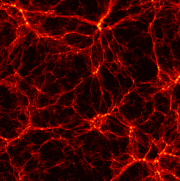
The Quijote Dark Matter simulations which we use as a dataset for our GNN.

Finally, we apply our approach to a real-world problem: dark matter in cosmology. Cosmology studies the evolution of the Universe from the Big Bang to the complex structures like galaxies and stars that we see today. The interactions of various types of matter and energy drive this evolution, though dark matter alone consists of ~85% of the total matter in the Universe (Spergel et al., 2003). Dark matter spurs the development of galaxies. Dark matter particles clump together and act as gravitational basins called “dark matter halos” which pull regular baryonic matter together to produce stars, and form larger structures such as filaments and galaxies. An important challenge in cosmology is to infer properties of dark matter halos based on their “environment”— the nearby dark matter halos. Here we study the problem: how can we predict the excess amount of matter, \(\delta_i\), in a halo \(i\) using only its properties and those of its neighbor halos?

We employ the same GNN model as before, only now we predict the overdensity of a halo instead of the instantaneous acceleration of particles. Each halo has connections (edges) in the graph to all halos within a 50 Mpc/h radius. The GNN learns this relation accurately, beating the following hand-designed analytic model:

\[\hat{\delta}_i = C_1 + (C_2 + M_i C_3) \sum_{j\neq i}^{\lvert\mathbf{r}_i - \mathbf{r}_j\rvert < 20 \text{ Mpc/h}} M_j,\]

where \(\mathbf{r}_i\) is position, \(M_i\) is mass, and \(C_{1:3}\) are constants.

Upon inspection, the messages passed within this GNN only possess a single significant feature, meaning that the GNN has learned it only needs to sum a function over neighbors (much like the hand-designed formula). We then fit the node function and message function, each of which output a scalar, and find a new analytic equation to describe the overdensity of dark matter given its environment:

\[\hat{\delta}_i = C_1 + \frac{1}{C_2 + C_3 M_i} \sum_{j\neq i} \frac{C_4 + M_j}{C_5 + (C_6 \lvert \mathbf{r}_i - \mathbf{r}_j \rvert)^{C_7}}\]

This achieves a mean absolute error of 0.088, while the hand-crafted analytic equation only gets 0.12. Remarkably, our algorithm has discovered an analytic equation which beats the one designed by scientists.

An illustration of how our technique learns a symbolic expression: first, a neural network undergoes supervised learning, then, symbolic regression approximates internal functions of the model.

Generalization

Given that symbolic models describe the universe so accurately, both for core physical theories and empirical models, perhaps by converting a neural network to an analytic equation, the model will generalize better. This is in some sense a prior on learned models.

Here we study this on the cosmology example by masking 20% of the data: halos which have \(\delta_i > 1\). We then proceed through the same training procedure as before. Interestingly, we obtain a functionally identical expression when extracting the formula from the graph network on this subset of the data. Then, we compare how well the GNN and symbolic expression generalize. The graph network itself obtains an average error of 0.0634 on the training set, and 0.142 on the out-of-distribution data. Meanwhile, the symbolic expression achieves 0.0811 on the training set, but 0.0892 on the out-of-distribution data. Therefore, for this problem, it seems a symbolic expression generalizes much better than the very graph neural network it was extracted from. This alludes back to Eugene Wigner’s article: the language of simple, symbolic models effectively describes the universe.